GPT：一个有限状态马尔可夫链GPT是一个神经网络，它接受一些离散令牌序列，并预测序列中下一个令牌的概率。例如，如果只有两个令牌0和1，那么一个小型的二进制GPT可以告诉我们：

[0,1,0] ---> GPT ---> [P(0) = 20%, P(1) = 80%]

在这里，GPT接受了位序列[0,1,0]，并基于当前参数设置，预测下一个数字是1的概率为80%。重要的是，默认情况下，GPT具有有限的上下文长度。例如，如果上下文长度为3，则它们只能输入最多3个标记。在上面的例子中，如果我们翻转一个有偏差的硬币并采样1确实会出现，那么我们将从原始状态[0,1,0]转换为新状态[1,0,1]。我们在右侧添加了新的位（1），并通过丢弃最左侧的位（0）将序列截断为上下文长度3。然后，我们可以一遍又一遍地重复这个过程来在状态之间进行转换。显然，GPT是一个有限状态马尔可夫链：有一组有限的状态和它们之间的概率转移箭头。每个状态由输入到GPT的标记身份的特定设置（例如[0,1,0]）定义。我们可以通过一定的概率转换到新状态，如[1,0,1]。让我们详细看看这是如何工作的。

# hyperparameters for our GPT
# vocab size is 2, so we only have two possible tokens: 0,1
vocab_size = 2
# context length is 3, so we take 3 bits to predict the next bit probability
context_length = 3

GPT神经网络的输入是一系列token序列。这些令牌是离散的，因此状态空间为：

print('state space (for this exercise) = ', vocab_size ** context_length)

详细说明：准确地说，GPT可以从1到context_length接受任意数量的标记。因此，如果上下文长度为3，我们原则上可以在尝试预测下一个标记时提供1个标记、2个标记或3个标记。在这里，我们将忽略这一点，并假设上下文长度已经“最大化”，以简化下面的一些代码。

用pytorch实现一个最小化GPT：

#@title minimal GPT implementation in PyTorch (optional)
""" super minimal decoder-only gpt """

import math
from dataclasses import dataclass
import torch
import torch.nn as nn
from torch.nn import functional as F


torch.manual_seed(1337)

class CausalSelfAttention(nn.Module):
  def __init__(self, config):
    super().__init__()
    assert config.n_embd % config.n_head == 0
    # key, query, value projections for all heads, but in a batch
    self.c_attn = nn.Linear(config.n_embd, 3 * config.n_embd, bias=config.bias)
    # output projection
    self.c_proj = nn.Linear(config.n_embd, config.n_embd, bias=config.bias)
    # regularization
    self.n_head = config.n_head
    self.n_embd = config.n_embd
    self.register_buffer("bias", torch.tril(torch.ones(config.block_size, config.block_size))
    .view(1, 1, config.block_size, config.block_size))
  def forward(self, x):
    B, T, C = x.size() # batch size, sequence length, embedding dimensionality (n_embd)
    # calculate query, key, values for all heads in batch and move head forward to be the batch dim
    q, k ,v  = self.c_attn(x).split(self.n_embd, dim=2)
    k = k.view(B, T, self.n_head, C // self.n_head).transpose(1, 2) # (B, nh, T, hs)
    q = q.view(B, T, self.n_head, C // self.n_head).transpose(1, 2) # (B, nh, T, hs)
    v = v.view(B, T, self.n_head, C // self.n_head).transpose(1, 2) # (B, nh, T, hs)
    
    # manual implementation of attention
    att = (q @ k.transpose(-2, -1)) * (1.0 / math.sqrt(k.size(-1)))
    att = att.masked_fill(self.bias[:,:,:T,:T] == 0, float('-inf'))
    att = F.softmax(att, dim=-1)
    y = att @ v # (B, nh, T, T) x (B, nh, T, hs) -> (B, nh, T, hs)
    y = y.transpose(1, 2).contiguous().view(B, T, C) # re-assemble all head outputs side by side
    
    # output projection
    y = self.c_proj(y)
    return y

class MLP(nn.Module):
  def __init__(self, config):
    super().__init__()
    self.c_fc    = nn.Linear(config.n_embd, 4 * config.n_embd, bias=config.bias)
    self.c_proj  = nn.Linear(4 * config.n_embd, config.n_embd, bias=config.bias)
    self.nonlin = nn.GELU()
  def forward(self, x):
    x = self.c_fc(x)
    x = self.nonlin(x)
    x = self.c_proj(x)
    return x

class Block(nn.Module):
  def __init__(self, config):
    super().__init__()
    self.ln_1 = nn.LayerNorm(config.n_embd)
    self.attn = CausalSelfAttention(config)
    self.ln_2 = nn.LayerNorm(config.n_embd)
    self.mlp = MLP(config)
  def forward(self, x):
    x = x + self.attn(self.ln_1(x))
    x = x + self.mlp(self.ln_2(x))
    return x

@dataclass
class GPTConfig:
  # these are default GPT-2 hyperparameters
  block_size: int = 1024
  vocab_size: int = 50304
  n_layer: int = 12
  n_head: int = 12
  n_embd: int = 768
  bias: bool = False

class GPT(nn.Module):
  def __init__(self, config):
    super().__init__()
    assert config.vocab_size is not None
    assert config.block_size is not None
    self.config = config
  
    self.transformer = nn.ModuleDict(dict(
    wte = nn.Embedding(config.vocab_size, config.n_embd),
    wpe = nn.Embedding(config.block_size, config.n_embd),
    h = nn.ModuleList([Block(config) for _ in range(config.n_layer)]),
    ln_f = nn.LayerNorm(config.n_embd),
    ))
    self.lm_head = nn.Linear(config.n_embd, config.vocab_size, bias=False)
    self.transformer.wte.weight = self.lm_head.weight # https://paperswithcode.com/method/weight-tying
    
    # init all weights
    self.apply(self._init_weights)
    # apply special scaled init to the residual projections, per GPT-2 paper
    for pn, p in self.named_parameters():
    if pn.endswith('c_proj.weight'):
    torch.nn.init.normal_(p, mean=0.0, std=0.02/math.sqrt(2 * config.n_layer))
    
    # report number of parameters
    print("number of parameters: %d" % (sum(p.nelement() for p in self.parameters()),))
  def _init_weights(self, module):
    if isinstance(module, nn.Linear):
    torch.nn.init.normal_(module.weight, mean=0.0, std=0.02)
    if module.bias is not None:
    torch.nn.init.zeros_(module.bias)
    elif isinstance(module, nn.Embedding):
    torch.nn.init.normal_(module.weight, mean=0.0, std=0.02)
  def forward(self, idx):
    device = idx.device
    b, t = idx.size()
    assert t <= self.config.block_size, f"Cannot forward sequence of length {t}, block size is only {self.config.block_size}"
    pos = torch.arange(0, t, dtype=torch.long, device=device).unsqueeze(0) # shape (1, t)
    
    # forward the GPT model itself
    tok_emb = self.transformer.wte(idx) # token embeddings of shape (b, t, n_embd)
    pos_emb = self.transformer.wpe(pos) # position embeddings of shape (1, t, n_embd)
    x = tok_emb + pos_emb
    for block in self.transformer.h:
    x = block(x)
    x = self.transformer.ln_f(x)
    logits = self.lm_head(x[:, -1, :]) # note: only returning logits at the last time step (-1), output is 2D (b, vocab_size)
    return logits

基于以上功能构造一个GPT对象：

config = GPTConfig(
  block_size = context_length,
  vocab_size = vocab_size,
  n_layer = 4,
  n_head = 4,
  n_embd = 16,
  bias = False,
)
gpt = GPT(config)

number of parameters: 12656

n_layer，n_head，n_embd，bias，这些是实现GPT的Transformer神经网络的一些超参数。

GPT的参数(12,656个)是随机初始化的，它们参数化了状态之间的转换概率。如果你顺利地改变这些参数，你将顺利地影响状态之间的转换概率。

现在让我们使用随机初始化的GPT。让我们将所有可能的输入输入到上下文长度为3的最小二进制GPT中:

def all_possible(n, k):
  # return all possible lists of k elements, each in range of [0,n)
  if k == 0:
    yield []
  else:
    for i in range(n):
    for c in all_possible(n, k - 1):
    yield [i] + c
list(all_possible(vocab_size, context_length)

[[0, 0, 0],
 [0, 0, 1],
 [0, 1, 0],
 [0, 1, 1],
 [1, 0, 0],
 [1, 0, 1],
 [1, 1, 0],
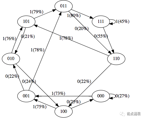
 [1, 1, 1]]

这8种可能性是GPT可能处于的8种状态。因此，让我们在每个可能的令牌序列上运行GPT，并获得该序列中下一个令牌的概率，并绘制成一个漂亮的图形:

# we'll use graphviz for pretty plotting the current state of the GPT
from graphviz import Digraph

def plot_model():
  dot = Digraph(comment='Baby GPT', engine='circo')

  for xi in all_possible(gpt.config.vocab_size, gpt.config.block_size):
    # forward the GPT and get probabilities for next token
    x = torch.tensor(xi, dtype=torch.long)[None, ...] # turn the list into a torch tensor and add a batch dimension
    logits = gpt(x) # forward the gpt neural net
    probs = nn.functional.softmax(logits, dim=-1) # get the probabilities
    y = probs[0].tolist() # remove the batch dimension and unpack the tensor into simple list
    print(f"input {xi} ---> {y}")
        
    # also build up the transition graph for plotting later
    current_node_signature = "".join(str(d) for d in xi)
    dot.node(current_node_signature)
    for t in range(gpt.config.vocab_size):
      next_node = xi[1:] + [t] # crop the context and append the next character
      next_node_signature = "".join(str(d) for d in next_node)
      p = y[t]
      label=f"{t}({p*100:.0f}%)"
      dot.edge(current_node_signature, next_node_signature, label=label)
  return dot

plot_model()


input [0, 0, 0] ---> [0.4963349997997284, 0.5036649107933044]
input [0, 0, 1] ---> [0.4515703618526459, 0.5484296679496765]
input [0, 1, 0] ---> [0.49648362398147583, 0.5035163760185242]
input [0, 1, 1] ---> [0.45181113481521606, 0.5481888651847839]
input [1, 0, 0] ---> [0.4961162209510803, 0.5038837194442749]
input [1, 0, 1] ---> [0.4517717957496643, 0.5482282042503357]
input [1, 1, 0] ---> [0.4962802827358246, 0.5037197470664978]
input [1, 1, 1] ---> [0.4520467519760132, 0.5479532480239868]

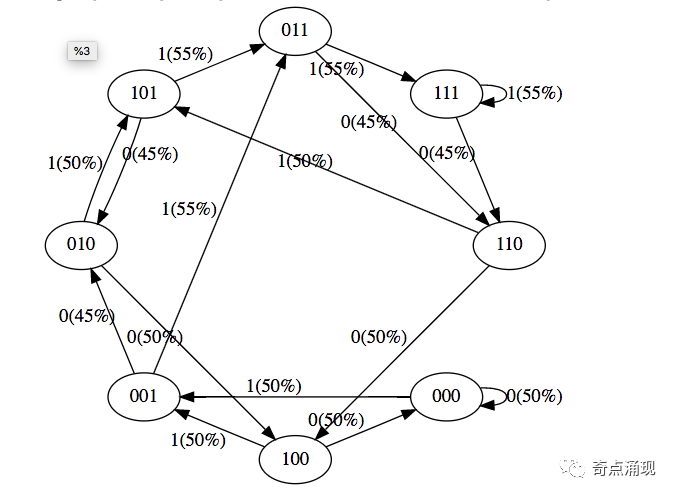
我们看到了8种状态，以及连接它们的概率箭头。因为有两种可能的标记，所以每个节点有两种可能的箭头。请注意，每次我们通过边进行“转换”时，最左边的令牌会被删除，而该边上的令牌会被追加到右边。请注意，在初始化时，大多数概率都是一致的(在本例中为50%)，这是很好的和理想的，因为我们甚至根本没有训练过模型。

# let's train our baby GPT on this sequence
seq = list(map(int, "111101111011110"))
seq
[1, 1, 1, 1, 0, 1, 1, 1, 1, 0, 1, 1, 1, 1, 0]

# convert the sequence to a tensor holding all the individual examples in that sequence
X, Y = [], []
# iterate over the sequence and grab every consecutive 3 bits
# the correct label for what's next is the next bit at each position
for i in range(len(seq) - context_length):
  X.append(seq[i:i+context_length])
  Y.append(seq[i+context_length])
  print(f"example {i+1:2d}: {X[-1]} --> {Y[-1]}")
X = torch.tensor(X, dtype=torch.long)
Y = torch.tensor(Y, dtype=torch.long)
print(X.shape, Y.shape)

example  1: [1, 1, 1] --> 1
example  2: [1, 1, 1] --> 0
example  3: [1, 1, 0] --> 1
example  4: [1, 0, 1] --> 1
example  5: [0, 1, 1] --> 1
example  6: [1, 1, 1] --> 1
example  7: [1, 1, 1] --> 0
example  8: [1, 1, 0] --> 1
example  9: [1, 0, 1] --> 1
example 10: [0, 1, 1] --> 1
example 11: [1, 1, 1] --> 1
example 12: [1, 1, 1] --> 0
torch.Size([12, 3]) torch.Size([12])

（未完，评论中继续）